
Natural Variability, Attribution and Climate Models #7
Estimates of Natural Variability over Long Timescales

In #6 we looked in a bit more detail at Imbers and co-authors from 2014. Natural variability is a big topic.
In this article we’ll look at papers that try to assess natural variability over long timescales - Peter Huybers & William Curry from 2006 who also cited an interesting paper from Jon Pelletier from 1998.
Here’s Jon Pelletier:
Understanding more about the natural variability of climate is essential for an accurate assessment of the human influence on climate. For example, an accurate model of natural variability would enable climatologists to make quantitative estimates of the likelihood that the observed warming trend is anthropogenically induced.
He notes another paper with this comment (explained in simpler terms below):
However, their stochastic model for the natural variability of climate was an autoregressive model which had an exponential autocorrelation dependence on time lag. We present evidence for a power-law autocorrelation function, implying larger low-frequency fluctuations than those produced by an autoregressive stochastic model. This evidence suggests that the statistical likelihood of the observed warming trend being larger than that expected from natural variations of the climate system must be reexamined.
In plain language, the paper he refers to used the simplest model of random noise with persistence, the AR(1) model we looked at in the last article.
He is saying that this simple model is “too kind” when trying to weigh up anthropogenic vs natural variations in temperature.
In other words, clearly the real world doesn’t match AR(1). It’s more complicated.
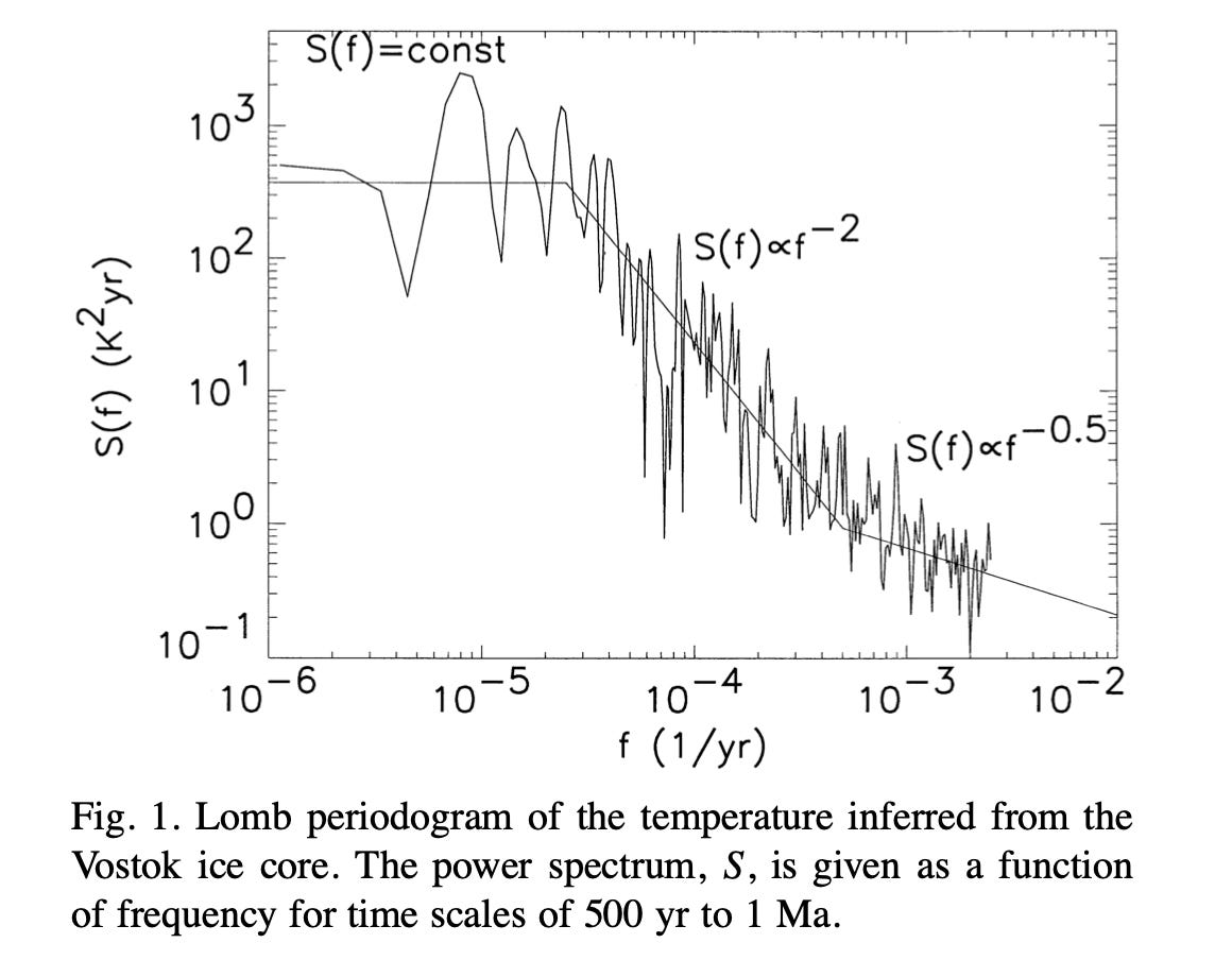
One very long dataset is temperature over the last million years inferred from an Antarctic ice core. The graph won’t mean a lot to many readers but I’ll explain the ideas in the background below:
If you’re familiar with spectral analysis you can skip the next section.
Background - explaining Spectral Analysis
Most people are familiar with the idea of a perfect pitch. Someone sings a perfect middle C, for example. The note sounds pure. Here’s what it looks like on a time axis:

This is a sine wave. It’s exactly one frequency. Instead of plotting it on a time axis you can plot it against frequency and it’s just one line at 261Hz.
To make sense of a signal, the frequency plot is often more revealing. Here’s an example of specific frequencies plus random noise:

It’s not obvious that this was built from a 50Hz signal, a 120Hz signal and some noise. But if we do a frequency analysis (using Fourier analysis), we can see it clearly:

Frequency analysis is very useful in physics and engineering.
Here’s another example that’s useful to know. This is “white noise”, 10,000 values plotted against time, each value is just a random number uncorrelated to the one before:
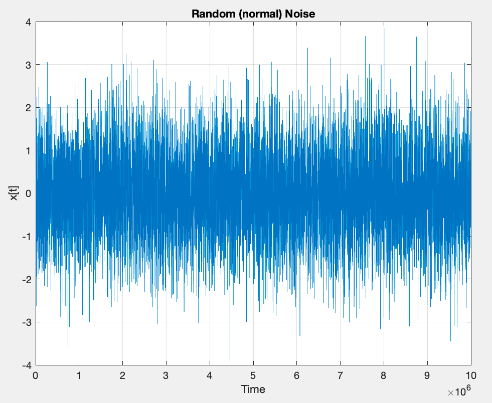
Here’s the spectrum of this data:
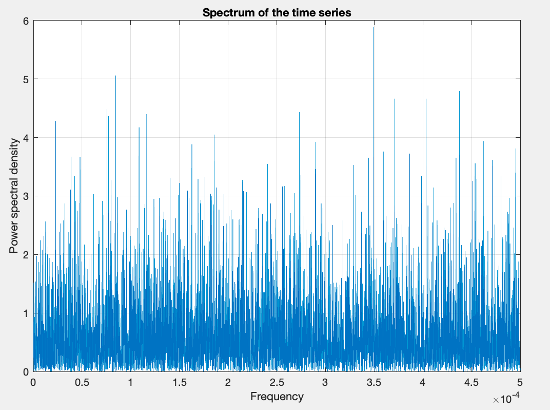
It doesn’t look very interesting or very different. But the spectrum of uncorrelated random noise is flat. Once we start adding persistence we get a spectrum with more energy at lower frequencies. Here’s the time series of an AR(1) process with a fairly high correlation (each value is 0.8 of the last value plus random noise):
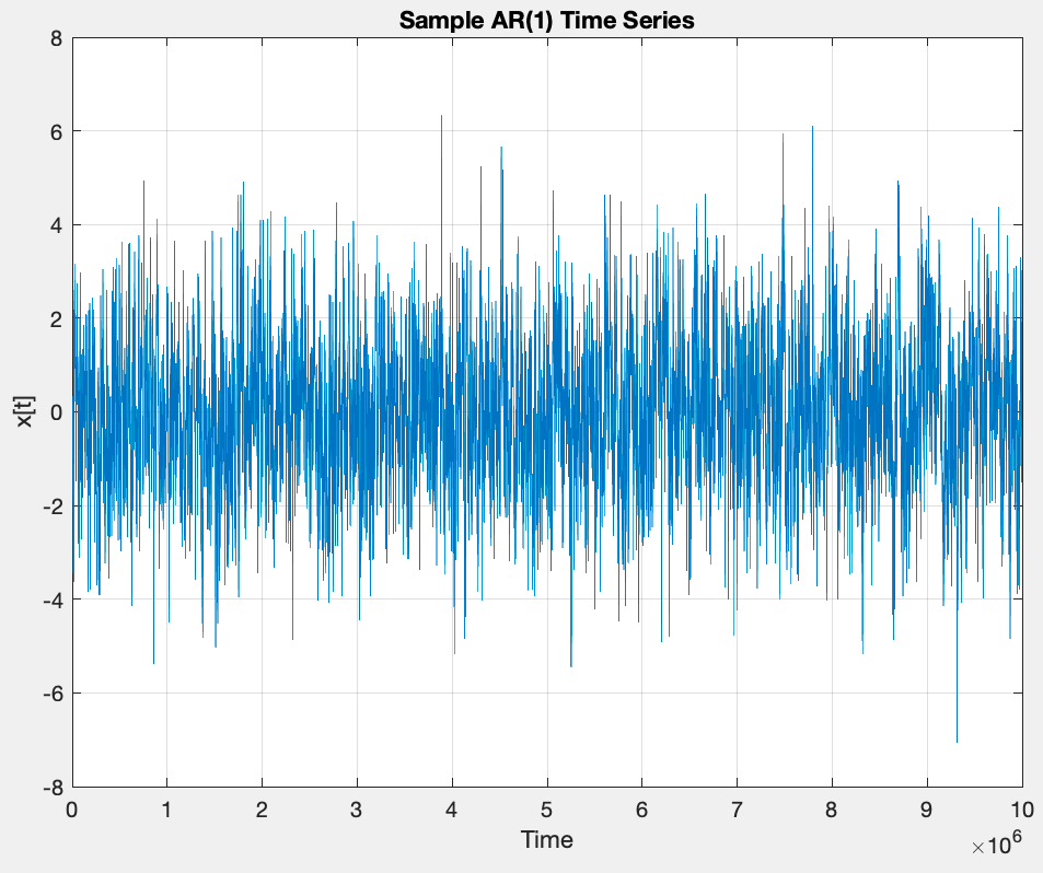
Zoomed in:

And now the spectrum:

You can see that there is more energy on longer timescales (lower frequency). The shape of this spectrum is what we are looking for, and that’s what both papers are about.
End of Background
Here’s the plot from Pelletier again, with annotation of time (frequency is 1/time) in red:
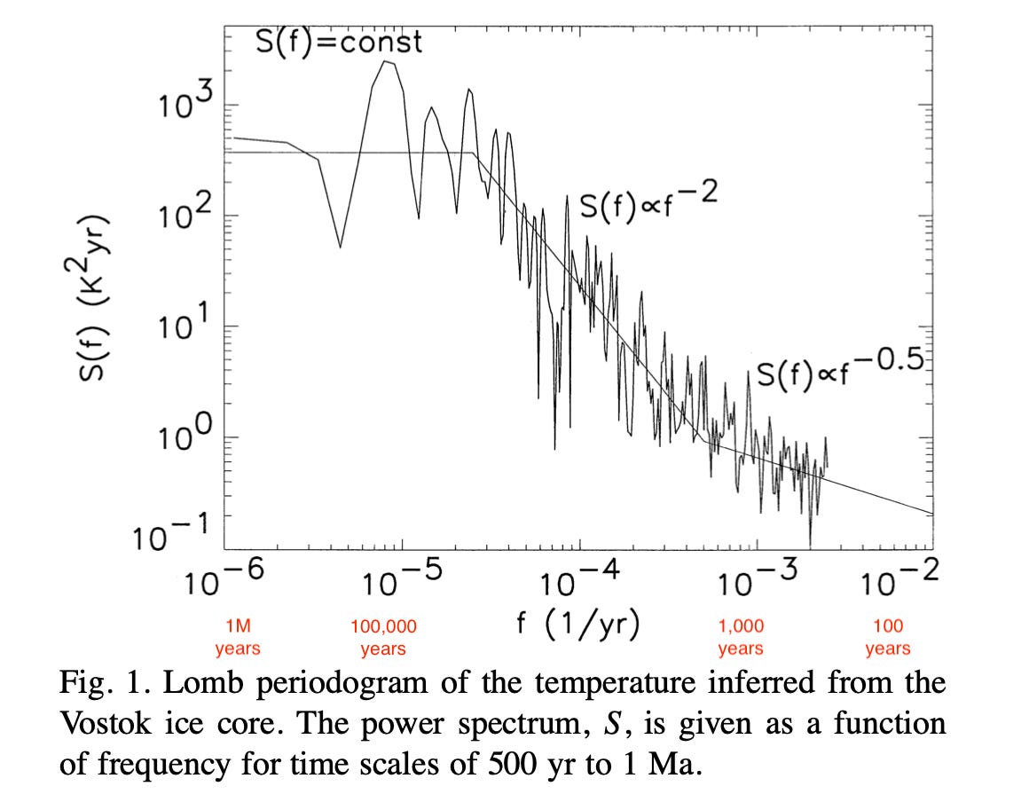
This is a log plot, so each major tick is 10x the frequency, or one tenth of the time. The energy value on the left axis is also a log scale so each major tick is 10x the energy of the value below.
We can see that different timescales seem to have different “power law” relationships.
What do we have apart from ice cores? The longest time series with a thermometer is 250 years from central England. We can see that the slope of the graph in this time range is similar to the ice core data at the shorter time periods:
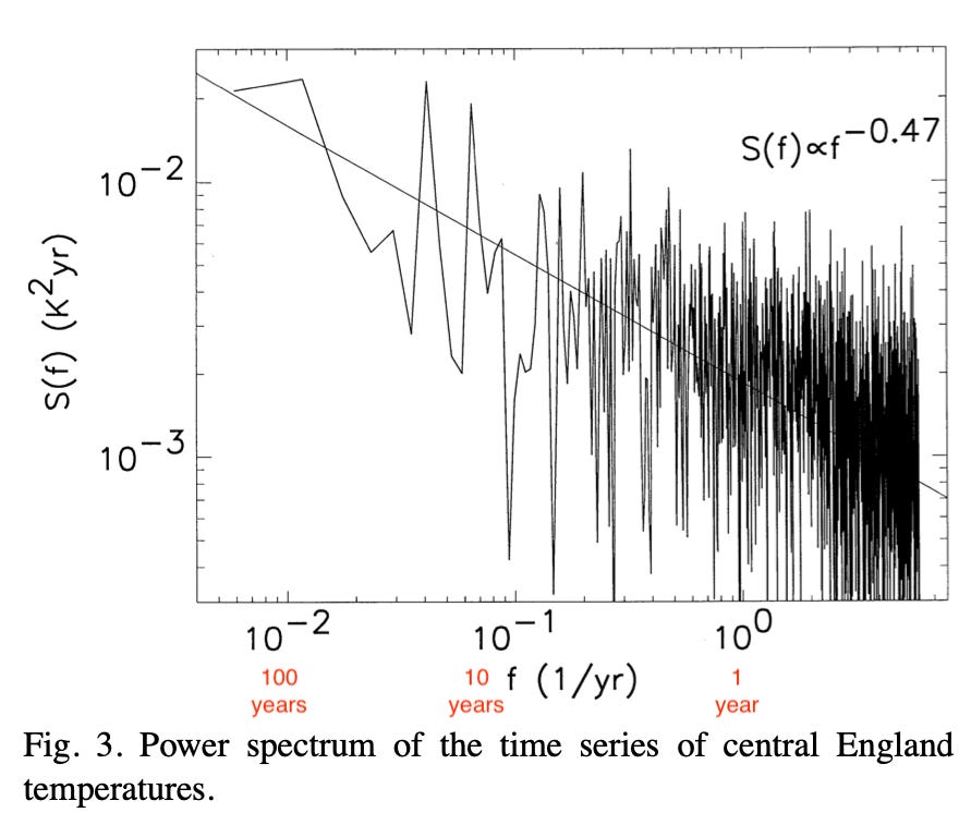
Note that he removed the annual signal which is very strong, and I added the red annotation to make it easier to read the time scale.
He also looked at shorter timescales - 10 years - with data from lots of weather stations and compared the spectra from ocean vs land stations and tried to build a simple physics model to explain the persistence.
Now onto Peter Huybers & William Curry from 2006. They describe the obvious record we see in long term climate data (primarily from ice cores and ocean data) which has an annual cycle and what are called Milankovitch cycles.
I did a whole series about the ice ages on the old blog - Ghosts of Climates Past.
In the briefest terms, we can see that ice sheets grew and shrank with frequencies that matched the changes in the orbital tilt of the earth.
As a small digression, there’s a huge sticking point explaining what caused ice ages to start and stop. Here’s George Kukla et al (2002) – written with a cast of eminents such as Shackleton, Imbrie & Broecker:
At the end of the last interglacial period, over 100,000 yr ago, the Earth’s environments, similar to those of today, switched into a profoundly colder glacial mode. Glaciers grew, sea level dropped, and deserts expanded. The same transition occurred many times earlier, linked to periodic shifts of the Earth’s orbit around the Sun. The mechanism of this change, the most important puzzle of climatology, remains unsolved.
But it does seem clear that the waxing and waning of ice sheets (not the start and end of the ice ages) can be explained as “orbital forcing” or “Milankovitch cycles”.
Huybers and Curry:
Relative to the annual and Milankovitch cycles, the continuum of climate variability has received little attention, but is nonetheless expected to embody a rich set of physical processes..
..The continuum can be described using spectral power laws: P(f) ∝ f-b, where P is spectral energy, f is frequency, and b is the power law. Power laws arise in physical systems as a result of nonlinearities transferring energy between different modes.
This is the same relationship as in Pelletier’s paper. The idea is to identify the value “b” over different timescales.
At interannual and decadal timescales, surface temperatures exhibit a strong land–sea contrast, with b averaging one over the oceans and zero over the continents.
At millennial and longer timescales, ice-core and marine palaeoclimate records indicate b is closer to two. Thus, long-period temperature variability has a larger b than does short-period variability, with a transition occurring near centennial timescales.
And then the key point - we can characterize it, but we need some idea grounded in physics to explain it:
Numerous explanations have been advanced regarding the continuum, including stochastic resonance, modified random walks, and diffusion, but all these models are partial descriptions of the variability. Ultimately, one seeks a physics of climate from which the temperature spectrum can be deduced, something analogous to oceanography’s theories for tides and internal waves. Further analysis of the continuum is expected to aid in distinguishing the processes that control climate change.
They look at high latitude continental records over 1M years and find similar relationships to Pelletier. They look at instrument data over 100 years and find that the tropical ocean has a different relationship than land and high latitude oceans.
Discussion of long-term climate variability is commonly divided between deterministic and stochastic components —often associated with spectral peaks and the continuum, respectively. The analysis presented here indicates that the annual and Milankovitch energy are linked with the continuum, and together represent the climate response to insolation forcing.
These observations have implications for understanding future climate variability. The distinction between the magnitude of low- and high-latitude climate variability may become smaller toward centennial timescales. Furthermore, the physics controlling centennial and longer-timescale temperature variability appears to be distinct from that of shorter timescales, raising questions of whether climate models able to represent decadal variations will adequately represent the physics of centennial and longer-timescale climate variability.
Lots of interesting questions along with some data. This article isn’t solving any major puzzles, we’re just putting a few jigsaw pieces onto the map.
Just to reiterate, it’s clear that the simplest model of persistence (AR1), often used as a basis for interpreting natural variability, is a long way from reality.
Note for commenters - for those who don’t understand radiative physics but think they do and want to yet again derail comment threads with how adding CO2 to the atmosphere doesn’t change the surface temperature.. head over to Digression #3 - The "Greenhouse effect" and add your comments there. Comments here on that point will be deleted.
References
Links between annual, Milankovitch and continuum temperature variability, Peter Huybers & William Curry, Nature (2006)
The power spectral density of atmospheric temperature from time scales of 10-² to 10⁶ yr, Jon D. Pelletier, Earth and Planetary Science Letters (1998)
One thing to note about the statistics of processes with persistence: the variance increases as the lenght of time being averaged increases. This means that 'stable climate' is an oxymoron. There is no such animal, at least in the length of time significant to humans. Now the really long term plot from the Vostok ice core shows that the variance may be constant when averaging over periods of 100,000 years or greater. But in geologic terms, that's recent history. Averaging over thirty years and calling that 'climate' rather than weather is something of a bad joke.
Note that I think that there is indeed an anthropogenic component from increased CO2 and other molecules with significant IR absorption/emission in the thermal IR in the recent temperature record, but it's not at all clear how big it is.